


HP vs TQ Theory

TECH Enthusiast
Joined: Apr 2009
Posts: 723
Likes: 4
You are very right - that would make things a lot easier. I got side tracked and need to get back to the model. I'm about to sit down and try to data from my previous engine configurations and see how that goes.
I have gone back through and made things a bit more generic. Added fields for:
CID
Bore (in)
Stroke (in)
SCR
DCR
EV diameter (in)
IV diameter (in)
NumCylinders
Expansion ratio (basically a DCR in reverse using the EVO event)
Piston weight (g)
Rod weight (g)
MassP&R (lbs)
In part, this has to do with the ability to make subtle changes later on and test the model against known configurations.
TECH Addict
Joined: Jul 2013
Posts: 2,189
Likes: 123
From: Portland, Oregon
Rod ratio also plays a role in whether the force being created is going into pushing the piston down/turning the crank/being converted into work, or if it's being wasted by pushing the piston sideways against the cylinder walls and just turning into heat/friction.
Thread Starter
Joined: Jul 2014
Posts: 10,450
Likes: 1,873
From: My own internal universe
As it pertains to the modeling a base calculation of rod/stroke ratio should be part of the calculation. That determines piston decel, dwell & accel rates. Decel & accel rates will vary as the crank goes through it's circular range of motion based on the rod/stroke ratio.
OK, so for the non-physics folks who might be reading this, when we say "adiabatic", what we are saying is that the total heat in the system is constant other than what is added or extracted on purpose (short version to keep it relatively simple). In reality, there is something called an adiabatic curve that and engine could theoretically follow if it were perfect. A quick example is the compression stroke. Imagine compressing the air, and all the pressure and temperature changes stayed in the air with no bleed off, and no heat loss. Not gonna happen, but that's the basic concept.
There are a lot of things I'll never be able to accurately calculate, but I don't think it will turn out to be necessary once they are at least accounted for. For example, during the power stroke, a ton of energy goes through the heads straight to the coolant and does no work. I may never get that number, but I might still be able to account for it by first getting the data points that I can account for.
Which is why I started with parasitic acceleration. That can be calculated pretty close. Where I'm still reworking is that there is a dual wave function going on, and I'm not sure yet what function to assign the second wave. Using the rod/stroke ratio is only part of it, because the angle makes a tremendous difference as well. I need to figure out the correct function and then integrate both over crank angle rotation and then divide by 2Pi to get the average acceleration. It was easy with sinusoidal only function, but I'm still working this one out.
I've also started working on fueling, and I'm actually very comfortable with how this is coming out. I started with the VE's and after a ton of unit conversion - using a straight 12.8 AFR (which was my dyno session) - I got 70% duty cycle at 7200 RPM. On my HPT logs, 70% is right about where I seem to max out on repeated runs. So, the first go on fueling looks to be within a few percent, which gives some raw energy inputs to start working with. I want to look more at the logs and compare before posting these equations.
My method was to take the VE and cylinder volume, RPMs, and air density to get grams of air per second. Then use AFR to get grams per second of fuel. Then use the heat of combustion of gasoline to get the total heat input to the system - assuming perfect combustion to CO2 and H2O. Then, convert KJ/S to KW (1:1) to HP to get into the same units.
I'm netting 1095 HP of energy input to extract 438 HP out according to the model at peak power - 6800 rpm.
I'm netting 787 HP of energy input to extract 379 HP out according to the model at peak TQ - 4800 rpm.
Thread Starter
Joined: Jul 2014
Posts: 10,450
Likes: 1,873
From: My own internal universe
I can say this much...
No matter how I try to run the calculations, air and fuel definitely continue to rise after peak power. I have to modify the VE's to fall off the face of the earth to get air and fuel to decrease immediately after peak power, but then I start to get efficiencies that are way too high and the power output falls far faster than the dyno curve actually does. In other words, I have to force the model using known erroneous/false data to make the airflow and fuel fall off after peak power
It is almost certainly internal resistances adding up.
TECH Addict
Joined: Jul 2013
Posts: 2,189
Likes: 123
From: Portland, Oregon
Your fuel calculations look very promising. And closely support your calculations for the horsepower required to spin the rotating assembly at those rpms. So at least the work you have done so far seems to be checking out. Either you're getting close to correct, or both sides are equally wrong together, either way you are consistent.
TECH Enthusiast
Joined: Apr 2009
Posts: 723
Likes: 4
I can say this much...
No matter how I try to run the calculations, air and fuel definitely continue to rise after peak power. I have to modify the VE's to fall off the face of the earth to get air and fuel to decrease immediately after peak power, but then I start to get efficiencies that are way too high and the power output falls far faster than the dyno curve actually does. In other words, I have to force the model using known erroneous/false data to make the airflow and fuel fall off after peak power
It is almost certainly internal resistances adding up.
No matter how I try to run the calculations, air and fuel definitely continue to rise after peak power. I have to modify the VE's to fall off the face of the earth to get air and fuel to decrease immediately after peak power, but then I start to get efficiencies that are way too high and the power output falls far faster than the dyno curve actually does. In other words, I have to force the model using known erroneous/false data to make the airflow and fuel fall off after peak power
It is almost certainly internal resistances adding up.
The farther from optimal the model becomes the larger the exponent of calculated error will be. What the actual error is can range from a squared to a cubed function across the range of BSFC.
To further add to your comments on adiabatic function for those not in the know, they can start here https://en.m.wikipedia.org/wiki/Adiabatic_invariant
Furthermore, The model of adiabatic function is a square. Time a linear measurement, energy a vertical measurement. In other words the function of energy rise & drop would happen in zero time & the enthalpy would sustain, over time, as a constant. The Conclusion is that adiabetic function can only exist outside of space & time. The net result of complete loss of enthalpy would return to the energy level before the energy reaction begins, or ambient temp. That is 100% adiabetic, or .000 BSFC.
To compare the non-adiabatic curve of an ICE, by overlaying it BSFC map, in comparison to the hypothetical "square" of adiabatic operation shows how far off it is.
As it pertains here, we only need concern ourselves with as close to adiabatic as we can get, within the constraints of energy loss over time & in mechanical transfer ability of the engines design, & factoring in remaining enthalpy.
There has to be energy retention in the system for the ICE to continue to make power. This has to do with the fact we can't operate outside of space & time. The very upper limit, from the testing I have been educated on, that is around 800*F EGT. That is in that 5hp/ cu in power range, under stoich burn conditions, at a RPM equivalent to a hypothetical Compression ratio.
Last edited by gtfoxy; Nov 6, 2015 at 04:10 PM.
look, you can swap cams to give whatever characteristics you want, but on a single cam, overhead valve engine, once the cam is installed, the overlap is fixed. So, the point of my comparison wasn't "overlap can never change", but a cam at 1200 rpm with 12* overlap has completely different reversion characteristics vs 6800. And that overlap at 1200 that has all kinds of choppiness and short-circuiting, etc, at 6800 is likely not doing any of that, as there is barely enough time to get the air started moving. by the time you get enough overlap to start showing those types of behaviors at 6800, the overlap is going to be enormous, and the engine probably wouldn't even idle at 1200 rpm.
I understand the general reasonings behind choosing cams for NA vs Turbo, but I would imagine a turbo application that is spinning in the 8500 rpm range, you would need the overlap to be quite large. But again, in this scenario, at 8500 rpm, the overlap duration in milliseconds is quite small vs the duration at idle.
I understand the general reasonings behind choosing cams for NA vs Turbo, but I would imagine a turbo application that is spinning in the 8500 rpm range, you would need the overlap to be quite large. But again, in this scenario, at 8500 rpm, the overlap duration in milliseconds is quite small vs the duration at idle.
this is like restricting your theory and question to a single engine. Why can't you compare all engines on the planet? Use data from every combustion engine to shape your theory. Its like trying to learn about DNA by only comparing human Genomes. You MUST compare every available orgamism's genome to get the more accurate model. You MUST use data from all engine platforms, in all engine scenarios, from airplane to boat perspectives, with every available part possible. Science does this for DNA data- its called bioinformatics. We do not have such free easy facility for engineformatics (is that what it would be called?) where part data would add up to scientific literature.
Next, a performance engine near peak torque frequently experiences VE above 100%. If you are using 100% in the old fashioned equation it would put you at a 10% loss near redline because your initial reference was using 100 when it was actually 110%. So from your mathematical perspective you have been missing 10% and maybe also calling it "parasitic loss".
Many engines employ variable camshaft timing now, even while you drive some can adjust electronically for a flat VE curve. These engines, like the Honda S2000 engine, have a nearly flat VE curve across the board to redline. If the engine is prepared for the application there should not be a "magic brick wall" so much related to the weight or friction of the design, more likely there will be a valvetrain related or piston speed limit related problem first. In other words, a real racing engine has every element of friction reduced as much as feasible to maximize horsepower, in general, so in these applications the engine is prepared properly, and such "steadily increasing friction component forces" are going to be reduced per the application, as opposed to using too tight of clearances as in OEM engines, and causing OILING/FRICTION issues because of OIL FLOW related failures.
Last edited by kingtal0n; Nov 6, 2015 at 03:57 PM.
Thread Starter
Joined: Jul 2014
Posts: 10,450
Likes: 1,873
From: My own internal universe
Your fuel calculations look very promising. And closely support your calculations for the horsepower required to spin the rotating assembly at those rpms. So at least the work you have done so far seems to be checking out. Either you're getting close to correct, or both sides are equally wrong together, either way you are consistent.
I'm starting to really think it's getting close to correct. I put my previous cam's stuff - VE's, DCR, etc, and it was ground 9 degrees off, which is why I swapped it out. It accurately predicts a double hump torque curve, an early torque peak at 3600, and an early power peak. It is not correctly predicting the peak power RPM. the motor peaked at 5600, but it's calculating 6200.
LS1 Tech Stories
The Best V8 Stories One Small Block at Time

Gas Monkey Built a 6-Wheel Ferrari Testarossa With a Corvette LT4 Engine
Verdad Gallardo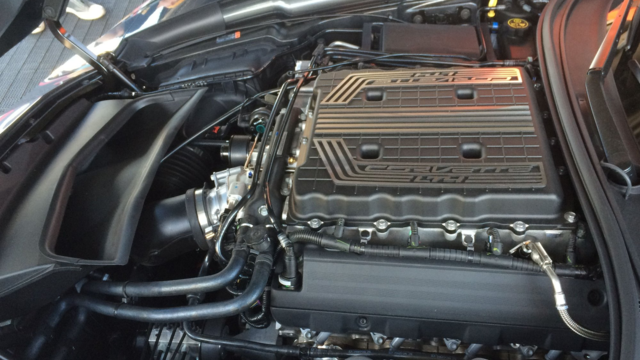
7 Most Reliable High-Performance Engines GM Has Ever Built
Verdad Gallardo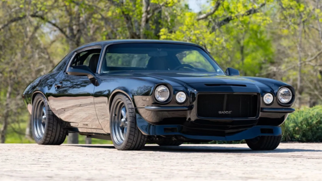
Amazing '71 Camaro Restomod Is Modern Muscle Car Under the Skin
Verdad Gallardo
6 Common C5 Corvette Failures and What's Involved In Repairing Them
Pouria Savadkouei
Retro Modern Bandit Pontiac Trans AM Comes With Burt Reynolds' Autograph
Verdad Gallardo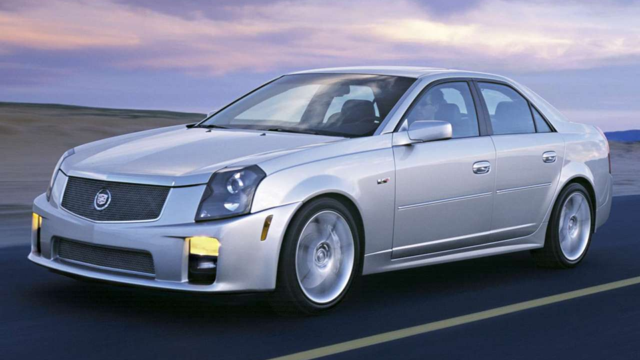
Top 10 Greatest Cadillac V Series Performance Models Ever, Ranked
Pouria Savadkouei
Top 10 Most Powerful Chevy Trucks Ever Made!

Hennessey's New Supercharged Silverado ZR2 Has 700 HP
Verdad Gallardo
Coachbuilt N2A Anteros Is an LS2-Powered C6 Corvette In Italian Clothes
Verdad Gallardo Thread Starter
Joined: Jul 2014
Posts: 10,450
Likes: 1,873
From: My own internal universe
Now you are talking about the resolution of error I was talking about. The parasitic loss you're trying to equate for, or are seeing/ not seeing, is due to ,as I said, the error in the sum of the whole as far as its scalar variance from a theoretical adiabetic function.
The farther from optimal the model becomes the larger the exponent of calculated error will be. What the actual error is can range from a squared to a cubed function across the range of BSFC.
The farther from optimal the model becomes the larger the exponent of calculated error will be. What the actual error is can range from a squared to a cubed function across the range of BSFC.
There comes a point, though, when you have to just use a number that gets you close. In the GM tune, there is a table that tells the computer the estimated friction losses at various RPM and MAP. So, GM got to that point as well, though admittedly their fudge factor will be pretty damned accurate compared to mine...
TECH Enthusiast
Joined: Apr 2009
Posts: 723
Likes: 4
Yes. And so many internet calculators expect you to just key in your BSFC as if you just sort of know it, so you can play with the number to make it give you what you want. I'm trying to actually back into my BSFC.
There comes a point, though, when you have to just use a number that gets you close. In the GM tune, there is a table that tells the computer the estimated friction losses at various RPM and MAP. So, GM got to that point as well, though admittedly their fudge factor will be pretty damned accurate compared to mine...
There comes a point, though, when you have to just use a number that gets you close. In the GM tune, there is a table that tells the computer the estimated friction losses at various RPM and MAP. So, GM got to that point as well, though admittedly their fudge factor will be pretty damned accurate compared to mine...
For simplification purposes a modern EFI motor will probably not exceed, in almost every normal application, .5BSFC. That would be the start to the model I would see as getting as close as you can to a hypothetical.
The base model I am talking about would be in the .3-.35 BSFC range. That is about our known limit at the moment. Hyper-scram Jet engines even exceed that number
Thread Starter
Joined: Jul 2014
Posts: 10,450
Likes: 1,873
From: My own internal universe
this is like restricting your theory and question to a single engine. Why can't you compare all engines on the planet? Use data from every combustion engine to shape your theory. Its like trying to learn about DNA by only comparing human Genomes. You MUST compare every available orgamism's genome to get the more accurate model. You MUST use data from all engine platforms, in all engine scenarios, from airplane to boat perspectives, with every available part possible. Science does this for DNA data- its called bioinformatics. We do not have such free easy facility for engineformatics (is that what it would be called?) where part data would add up to scientific literature.
Next, a performance engine near peak torque frequently experiences VE above 100%. If you are using 100% in the old fashioned equation it would put you at a 10% loss near redline because your initial reference was using 100 when it was actually 110%. So from your mathematical perspective you have been missing 10% and maybe also calling it "parasitic loss".
Many engines employ variable camshaft timing now, even while you drive some can adjust electronically for a flat VE curve. These engines, like the Honda S2000 engine, have a nearly flat VE curve across the board to redline. If the engine is prepared for the application there should not be a "magic brick wall" so much related to the weight or friction of the design, more likely there will be a valvetrain related or piston speed limit related problem first. In other words, a real racing engine has every element of friction reduced as much as feasible to maximize horsepower, in general, so in these applications the engine is prepared properly, and such "steadily increasing friction component forces" are going to be reduced per the application, as opposed to using too tight of clearances as in OEM engines, and causing OILING/FRICTION issues because of OIL FLOW related failures.
Second statement - I'm using my actual VE's, not estimates. They do exceed 100% from 4400 to 6400 RPM. Based on the AFR on the dyno at 12.6-12.9 AND the PE multiplier of 1.15, I'm getting exactly the wideband readings off the dyno I should get with the VE values in my table. My stock VE's are no good, because the car was never tuned on the stock cam. The VE table looks like stir-fried a$$ in the stock tune. Curious as to how GM ended up with those numbers.
Lastly, It's starting to look like friction is overall a linear function. I've got some more work to do on it, but it actually can be somewhat calculated. The main variable is the oil viscosity changes with temperature. Everything else in the friction system appears to be relatively constant. The side loading of the pistons will be tricky, because engine load will determine piston side loading. Tricky, because the angle on the crank is not equal to the angle on the rod. I don't think it will be flat like "60 all the way across" or something easy like that, but I do think it will simplify to a multivariate line.
Thread Starter
Joined: Jul 2014
Posts: 10,450
Likes: 1,873
From: My own internal universe
Well, I got the BSFC numbers, and they didn't make me hold my sides laughing or rush back to the drawing board.
I'm not going to count the low end, as I have this area deliberately lean - holding about 0.35 from idle to 3000. Starting at 3200 RPM, I'm at 0.4000 Lb/HpHr. From there, it is basically a steady rise to 0.508 Lb/HpHr at 6000 rpm. Then, it sort of jumps to 0.53 at 6400, 0.55 at 6800, and 0.58 at 7200.
TO me, that is a classic example of the law of diminishing returns - it is taking more effort to increase the engine speed a similar interval as the speed increases.
Thread Starter
Joined: Jul 2014
Posts: 10,450
Likes: 1,873
From: My own internal universe
I think this video is relevant to this discussion. Video Link: https://youtu.be/rBZCnG1HwDM It's long, but a good one.
Also, breaking it down to mean effective pressure might simplify a lot of this for me.
Good to see you posting, Martin!
Thread Starter
Joined: Jul 2014
Posts: 10,450
Likes: 1,873
From: My own internal universe
Thread Starter
Joined: Jul 2014
Posts: 10,450
Likes: 1,873
From: My own internal universe
@GTFoxy - is this what you were looking to see?
OK, I found a mistake since my previous post - I had used my calculated TQ/HP values instead of my actuals when I calculated BFSC. I redid it with the actuals, and it makes a lot more sense now:
RPM......HP......BFSC
2400...152......0.456
2800...184......0.448
3200...227......0.43
3600...267......0.43
4000...309......0.436
4400...345......0.452
4800...380......0.468
5200...412......0.475
5600...436......0.48
6000...456......0.482
6400...471......0.487
6800...471......0.509
But, you can see that in the data, peak HP was crossed between 6400 and 6800, but it requires more fuel to obtain 471 at 6800 vs 6400, indicating that adding energy is not increasing engine output.
The above is calculated BSFC vs actual HP. based on injector duty cycle logs, BFSC is calculating correctly.
Thread Starter
Joined: Jul 2014
Posts: 10,450
Likes: 1,873
From: My own internal universe
Another thought I had about this is that the VE is quite low at and near idle due to overlap. This came up earlier in this thread - losses out the pipe due to overlap. i think this is what is presenting on the low end. The cam really comes into itself around 3K and then pulls like a freight train. Martin discussed a similar phenomenon on his LSA thread. In this case, I think that around 3K, the overlap event is short enough in duration that the air and fuel quit short circuiting out the exhaust and the additional contribution to energy production begins. Past peak HP, I don't think that the overlap is magically getting longer in duration on the same cam, so I'm pretty sure the increasing losses are responsible at the high end.
The video Martin posted actually helped quite a bit to generalize things. They take the average effects for two revolutions and calculate the Mean Effective Pressure. That made it much easier to work with some of the numbers. I was able to somewhat generalize Brake Mean Effective Pressure, and there are two very distinct and obvious curves - one before peak TQ and one after peak TQ. When you see it, it becomes very obvious that the mechanisms affecting low RPM performance are not the same as those affecting high RPM performance. It is quite stark. I'll post a picture when my computer starts cooperating.

TECH Enthusiast
Joined: Apr 2009
Posts: 723
Likes: 4
@GTFoxy - is this what you were looking to see?
OK, I found a mistake since my previous post - I had used my calculated TQ/HP values instead of my actuals when I calculated BFSC. I redid it with the actuals, and it makes a lot more sense now:
RPM......HP......BFSC
2400...152......0.456
2800...184......0.448
3200...227......0.43
3600...267......0.43
4000...309......0.436
4400...345......0.452
4800...380......0.468
5200...412......0.475
5600...436......0.48
6000...456......0.482
6400...471......0.487
6800...471......0.509
But, you can see that in the data, peak HP was crossed between 6400 and 6800, but it requires more fuel to obtain 471 at 6800 vs 6400, indicating that adding energy is not increasing engine output.
The above is calculated BSFC vs actual HP. based on injector duty cycle logs, BFSC is calculating correctly.
OK, I found a mistake since my previous post - I had used my calculated TQ/HP values instead of my actuals when I calculated BFSC. I redid it with the actuals, and it makes a lot more sense now:
RPM......HP......BFSC
2400...152......0.456
2800...184......0.448
3200...227......0.43
3600...267......0.43
4000...309......0.436
4400...345......0.452
4800...380......0.468
5200...412......0.475
5600...436......0.48
6000...456......0.482
6400...471......0.487
6800...471......0.509
But, you can see that in the data, peak HP was crossed between 6400 and 6800, but it requires more fuel to obtain 471 at 6800 vs 6400, indicating that adding energy is not increasing engine output.
The above is calculated BSFC vs actual HP. based on injector duty cycle logs, BFSC is calculating correctly.